Prior Visualization

• Visualizing Prior Distributions
  • How do we do this?
  • What do we check?

Visualizing Prior Distributions

Dear Young Tim,

My last post to you was about priors for neural networks. Far from being out of the blue, that post was a product of two active streams of research. Specifically, I referenced deep learning in computer science and prior specification from statistics. In doing so, I made two main points. First, neural networks are a flexible way to parameterize one’s likelihood function. And second, we should complement neural network parameters with prior distributions. These priors provide regularization and enable posterior inference / uncertainty estimates for the parameters.

In this post, I’m going to focus on the statistician’s perspective. The broader stream of literature in statistics has converged on the following two points. First, instead of being uninformative as intended, vague / diffuse priors can be highly informative about functionals of one’s model, in ways that one may actively dislike. Second, the way to understand one’s prior is by spending a lot of time inspecting (i.e., visualizing) the prior predictive distribution.

This post will demonstrate the two points above by way of pictures and an example. For relevant reading that provides much of the inspiration for this post, see the following papers:

• Seaman III, John W., John W. Seaman Jr, and James D. Stamey. “Hidden dangers of specifying noninformative priors.” The American Statistician 66, no. 2 (2012): 77-84.
• Gelman, Andrew, Daniel Simpson, and Michael Betancourt. “The prior can often only be understood in the context of the likelihood.” Entropy 19, no. 10 (2017): 555.
• Gabry, Jonah, Daniel Simpson, Aki Vehtari, Michael Betancourt, and Andrew Gelman. “Visualization in Bayesian workflow.” Journal of the Royal Statistical Society: Series A (Statistics in Society) 182, no. 2 (2019): 389-402.

The conclusion for one’s own research is that when building models of any kind, one should spend time investigating and setting informative priors for one’s models by visualizing the prior predictive distribution.

Below, I’ll share some examples of such prior investigations using the widely available Boston Housing data set:

Harrison Jr, David, and Daniel L. Rubinfeld. “Hedonic housing prices and the demand for clean air.” (1978).

The model that we’ll consider is a folded-logistic regression model where the location is linearly parameterized based on the dataset’s raw features, and where the scale parameter is homogenous and explicitly estimated. Note that if $Z$ follows a logistic distribution with location $\mu$ and scale $\sigma$, then $\lvert Z \rvert$ follows a folded logistic distribution. Basically, this is a linear regression where we restrict the support of the outcome (i.e, the median home value) to positive real values, following a logistic distribution bounded below by zero.

How do we do this?

The general strategy for prior predictive checks is as follows.

1. Specify a prior distribution for all parameters in one’s model.
2. Sample parameters from the prior.
3. Simulate outcomes from the model, conditional on one’s sampled parameters.
4. Visualize select statistics based on the simulated outcomes and explanatory variables.

To streamline this process, we need an interactive way of specifying our priors. While many options for interactivity exist, I’ll make use of the Streamlit package in Python. This package is easy to use, is generally free of “gotchas,” and enables one to set up a user-interface for one’s programs in a short time.

The basic idea is that we’ll select distributions via drop-down menus, and we’ll select parameters for those distributions via sliders. Then, once we’ve made our selections, we can press “Draw” or some other descriptively named button. This button press will trigger execution of a program that we’ve written to sample from our prior predictive distribution and create the desired visualizations. Finally, we’ll use Streamlit to automatically display these visualizations.

What do we check?

For an example of the prior predictive checking process in action, see the following repository: https://github.com/timothyb0912/prior-elicitation/. In particular, the streamlit app that I created to visualize the prior predictive checks is here, and the file I created to simulate from and visualize the prior is here.

To begin, we’ll need to choose some quantities to visualize. Here, we have complete freedom. For a variety of quantities that may prove useful for prior (or posterior) predictive checks, see

Brathwaite, Timothy. “Check yourself before you wreck yourself: Assessing discrete choice models through predictive simulations.” arXiv preprint arXiv:1806.02307 (2018).

For this example, we’ll consider a statistic that was not described in my paper. Specifically, we’ll examine the 25th percentile of Y * X, where X is a selected column from our design matrix. For instance, if we select the column of one’s in the design matrix, then we’ll view the prior predictive distribution of the 25th percentile of Y.

Here’s a picture using a typical diffuse / non-informative prior. 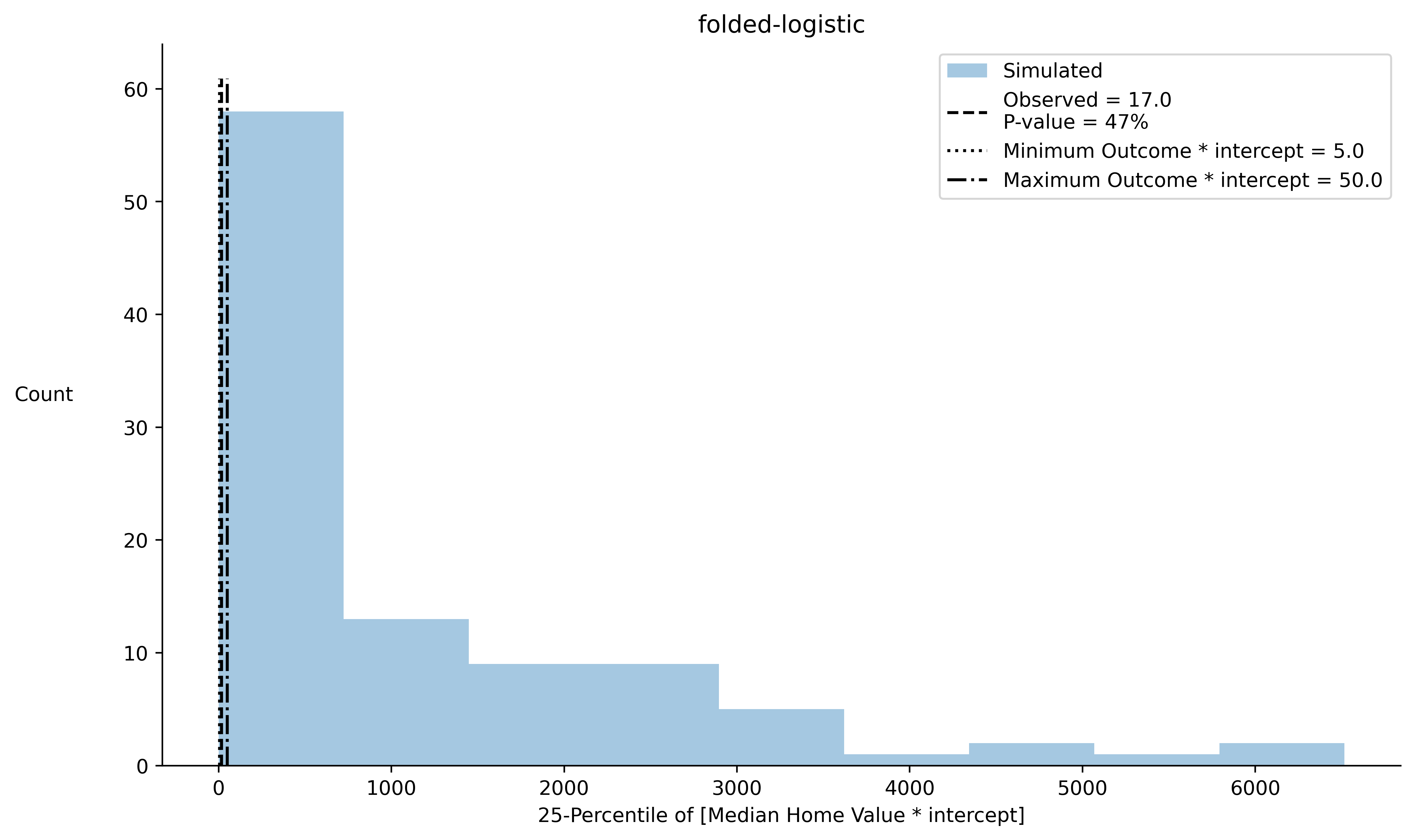Each coefficient for the design matrix has mean zero and standard deviation of 5. The scale parameter has a folded normal prior distribution with location 1 and scale of 1 (yes… meta, I know). From the image, we see that the prior predictive distribution places far too much mass on entirely implausible values (e.g. smaller than the minimum observed median home value or larger than the maximum observed median home value). The non-informative prior on the model parameters is actually quite opinionated (in misrepresentative ways) about our prior beliefs in functionals of our data.

From here, the idea is clear enough: play around! Iteratively adjust the sliders and display your chosen prior predictive checks for each new specification. With enough experimentation, one should be able to create a prior that appears reasonable.

See below for a video clip of how one can use the interactive interface to experiment with different prior settings.

In future posts, I’ll discuss how to set priors programmatically. Clearly, the manual approach described above will not scale to high dimensional settings. We’ll need to do something smarter!

P.S. The test statistic chosen for the prior predictive check has some rationale to it. In a standard linear regression, the first order conditions that one must solve to achieve a gradient of zero is $(Y - \hat{Y})X = 0$, where X is one’s design matrix. This is equivalent to saying that the mean of $YX$ should equal the mean of $\hat{Y}X$. In other words, the observed mean of $YX$ should equal the predicted $\hat{Y}X$ after estimating one’s model. Checking that the chosen test statistic of a selected percentile (e.g. 25th percentile) of $YX$ resembles the distribution of simulated $Y_{\textrm{sim}}X$ is a related activity. This helps ensure that more points of the distribution of $YX$ are well represented by one’s model, beyond the mean of the distribution.